i1Profiler .cxf Optimization Files
Device color profiles may be optimized by the addition of targeted color measurements. When profiling a device from scratch, a “volley” of colors is printed and measured, with the expectation that the gamut of the device will be fully represented. But if certain colors are of particular interest, such as grays and near-grays, more precise targeting may be of value, because it is not known in advance what the device’s actual response will be. RGB (127, 127, 127), for example, may not print as a neutral gray.
i1Profiler is able to optimize printer profiles by converting selected Lab colors to print values through an existing profile. This will help to ensure that colors of interest, such as grays, are accurately represented in the profile. The application will also select colors to “fill in the gaps” of the profile.
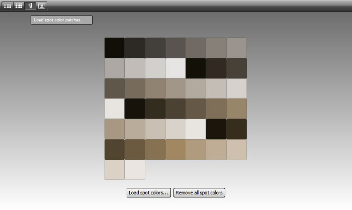
One first generates a set of Lab values in the form of a .cxf (color exchage format) file. The colors are then loaded as spot colors on the Patch Set page of i1Profiler’s printer optimization workflow. Select an existing profile, then click the third little button in the upper left of the patch set window (the one with a picture of a swatch set). Click Load spot colors, then navigate to the desired .cxf file. “Smart patches” to fill in gaps in the profile may also be generated (the number must be at least 50). Colors may also be extracted from an image, but the results may not be what one might expect. To see the sum of all the added colors, click the button with the sigma on it. One then prints the colors as a test chart and creates a new profile based on the old, “upgraded” with the addition of new measurements.
Display profiles may be similarly optimized, but the process is not formally identified as such. On the Patch Set page of the display profiling workflow, spot color Lab values are evidently run through the currently-active display profile, optimizing the selection of colors for profiling.
The optimization concept may be intepreted in different ways. On one hand, a high-quality profile may be fine-tuned to ensure that colors of interest are accurately represented. On the other hand, optimization may be incorporated into the workflow; a small, simple profile may be generated first, and used as the basis for more accurate selection of a larger number of colors, or specific colors for a specialized profile such as black-and-white or sepia. The value of optimizing a high-quality profile has been debated; after optimizing a profile originally created using 1000+ patches, the results are almost imperceptible. Neil Snape, for example, believes that optimization seems to be intended for profiles created with small patch sets.
I had wanted to optimize profiles for sepia tones and perhaps other colors such as cyanotypes, as well as small-gamut grays and near-grays. One way to do it is to select colors from an image in an image editor, such as a gradient colorized with a Hue/Saturation layer, or a duotone, and record their Lab values. Note that colors generated in this manner are device-specific, and depend on the color space (ProPhoto etc.) in which they are generated. Below are links to a number of generators that will produce .cxf files from both Lab and device-specific colors for optimization. The values are color managed for several color spaces. Browsers by specification display colors in sRGB; the generated color values are converted to sRGB patches for accurate display (within the limits of your monitor). Run the scripts, then save the output as regular ANSI-encoded text files with the extension .cxf. If the stylesheet cxf.xsl is in the same folder, you can open the .cxf files with a browser to see results formatted as in the illustration below. You may have to add an .xml extension to the files to get them to open in some browsers. You can also do this with i1Profiler’s patch sets such as .pxf (printer) or .dptf (monitor), but you have to add the stylesheet specification to the file (open it with a plain text editor such as Notepad or gedit, and add the second line below:)
<?xml version="1.0" encoding="UTF-8"?>
<?xml-stylesheet type="text/xsl" href="cxf.xsl"?>
.cxf File Generators
Lab: generates CIELab colors directly.
LCh (CIELCh, or Lightness, Chroma, hue): a cylindrical representation of CIELab, analogous to HSB or HSL.
Colorize/HSL: generates HSL (Hue, Saturation, Lightness) values in the same way that image editors do via “Colorize” or “Recolor.” Intended to imitate the appearance of a toned photograph or a duotone; the colors fade to white at the top, and black at the bottom.
HSB (Hue, Saturation, Brightness): colors tend to retain their hue all the way to the top and bottom; emphasizes pastel tints and rich shades.
RGB: maybe someone will find a use for this one. (Optimization in i1Profiler requires Lab values.)
Custom Lab: enter your own values and convert them to a .cxf file.
Stylesheet: cxf.xsl. If this file is in the same folder, you can open .cxf files with a browser to see formatted results as shown below. You may have to add an .xml extension to the files to get them to open in some browsers.
2023 UPDATE - this was true a long time ago; nowadays, the only browsers I have that still do it are Falkon and qutebrowser (go Qt !).
Sample .cxf file: LabGrays179.cxf.
Below is a set of HSL patches from a .cxf file, colorized with Hue = 50.
Source: Colorize/HSL ranges
Color space: ProPhoto2255 RGB
Patch count: 44
| H S L | L a b | |||||||
|---|---|---|---|---|---|---|---|---|
| No. | H | S | L | L* | a* | b* | ||
| 1 | 50 | 4 | 10 | 6.09573 | 0.32082 | 1.52125 | ||
| 2 | 50 | 4 | 18 | 17.73311 | 0.58940 | 2.95360 | ||
| 3 | 50 | 4 | 26 | 28.17436 | 0.77184 | 3.86781 | ||
| 4 | 50 | 4 | 34 | 37.77838 | 0.93964 | 4.70872 | ||
| 5 | 50 | 4 | 42 | 46.79224 | 1.09714 | 5.49795 | ||
| 6 | 50 | 4 | 50 | 55.35666 | 1.24678 | 6.24783 | ||
| 7 | 50 | 4 | 58 | 63.07730 | 1.00316 | 5.04145 | ||
| 8 | 50 | 4 | 66 | 70.53262 | 0.78093 | 3.94041 | ||
| 9 | 50 | 4 | 74 | 77.76105 | 0.57514 | 2.92029 | ||
| 10 | 50 | 4 | 82 | 84.79206 | 0.38241 | 1.96448 | ||
| 11 | 50 | 4 | 90 | 91.64893 | 0.20033 | 1.06116 | ||
| 12 | 50 | 8 | 10 | 6.50617 | 0.67662 | 3.02771 | ||
| 13 | 50 | 8 | 18 | 18.47383 | 1.18557 | 5.91709 | ||
| 14 | 50 | 8 | 26 | 29.14436 | 1.55254 | 7.74857 | ||
| 15 | 50 | 8 | 34 | 38.95926 | 1.89008 | 9.43320 | ||
| 16 | 50 | 8 | 42 | 48.17105 | 2.20687 | 11.01431 | ||
| 17 | 50 | 8 | 50 | 56.92353 | 2.50788 | 12.51659 | ||
| 18 | 50 | 8 | 58 | 64.34646 | 2.01991 | 10.09704 | ||
| 19 | 50 | 8 | 66 | 71.52767 | 1.57507 | 7.89116 | ||
| 20 | 50 | 8 | 74 | 78.50054 | 1.16346 | 5.84886 | ||
| 21 | 50 | 8 | 82 | 85.29098 | 0.77828 | 3.93626 | ||
| 22 | 50 | 8 | 90 | 91.91966 | 0.41466 | 2.12933 | ||
| 23 | 50 | 12 | 10 | 6.93132 | 1.06547 | 4.51882 | ||
| 24 | 50 | 12 | 18 | 19.20895 | 1.78306 | 8.88966 | ||
| 25 | 50 | 12 | 26 | 30.10701 | 2.33496 | 11.64124 | ||
| 26 | 50 | 12 | 34 | 40.13121 | 2.84261 | 14.17218 | ||
| 27 | 50 | 12 | 42 | 49.53943 | 3.31907 | 16.54760 | ||
| 28 | 50 | 12 | 50 | 58.47855 | 3.77176 | 18.80457 | ||
| 29 | 50 | 12 | 58 | 65.60854 | 3.03906 | 15.16300 | ||
| 30 | 50 | 12 | 66 | 72.51872 | 2.37090 | 11.84731 | ||
| 31 | 50 | 12 | 74 | 79.23798 | 1.75279 | 8.78003 | ||
| 32 | 50 | 12 | 82 | 85.78902 | 1.17462 | 5.90909 | ||
| 33 | 50 | 12 | 90 | 92.19015 | 0.62913 | 3.19777 | ||
| 34 | 50 | 16 | 10 | 7.37127 | 1.48764 | 5.99510 | ||
| 35 | 50 | 16 | 18 | 19.93866 | 2.38089 | 11.87264 | ||
| 36 | 50 | 16 | 26 | 31.06259 | 3.11783 | 15.54753 | ||
| 37 | 50 | 16 | 34 | 41.29454 | 3.79568 | 18.92774 | ||
| 38 | 50 | 16 | 42 | 50.89775 | 4.43188 | 22.10024 | ||
| 39 | 50 | 16 | 50 | 60.02214 | 5.03636 | 25.11456 | ||
| 40 | 50 | 16 | 58 | 66.86373 | 4.05961 | 20.24046 | ||
| 41 | 50 | 16 | 66 | 73.50586 | 3.16799 | 15.80932 | ||
| 42 | 50 | 16 | 74 | 79.97340 | 2.34296 | 11.71394 | ||
| 43 | 50 | 16 | 82 | 86.28621 | 1.57141 | 7.88300 | ||
| 44 | 50 | 16 | 90 | 92.46041 | 0.84373 | 4.26650 | ||