The icon generator
The equations
This script draws icon attractors based on equations described in Symmetry in Chaos by Michael Field and Martin Golubitsky. The image points are iterations of the following for the complex number z. For all the equations, n is an integer that determines the degree of symmetry, p is also an integer, and the rest are real numbers.
Icon 0: f(z) = λ(1 - zz̄)z +
γz̄n-1
This is actually a simplified version of Icon 1, where α = -λ, and β and ω are zero. It runs a little faster, fwiw.
Icon 1: f(z) = [λ + αzz̄ +
βRe(zn) + ωi]z +
γz̄n-1
For this and Icon 2, α and λ should have opposite signs. The ω parameter gives a “spin” to the image and changes the symmetry from radial to rotational.
Icon 2: f(z) = [λ + αzz̄ +
βRe(zn) +
δRe([z/|z|]np)|z|]z +
γz̄n-1
The p parameter tends to put angles and ripples into the image that increase as δ increases.
Generating the icons is an iterative process in more ways than one. The general approach is to find parameters for the equations that produce an interesting low-resolution image, then draw it at higher resolution and color it.
First: load an icon type and some parameters. A number of presets are included. Then start incrementing the parameters. The spin buttons next to the parameter felds increment the last decimal place of the displayed number; for larger or smaller increments, add or remove a digit. When “auto” is checked, the script will automatically quick draw a low-resolution image when a parameter is changed.
The equations only produce interesting images for certain parameters. Sometimes the equations run away to infinity; if this happens, the information field to the right will indicate “overflow.” If you hit an unproductive range of numbers, try increasing the increment and pressing on; you may find another useful range.
Sometimes a low-resolution image looks incomplete. As the points are generated, they fill in the image in chaotic fashion, and it may take more points to complete some images.
Next: when you want to generate a higher-resolution image, set the desired size, oversample level, and density, and click draw. Oversampling starts with an enlarged array of image points, then reduces it to the size of the final image. The net effect is the recording of points at the subpixel level for increased resolution. This comes at the expense of processing time and computer memory; oversampling by 4 means 16 times as many points. (Note that JavaScript is not as fast as lower-level programming languages.) “Density” refers to how many points are generated; it is proportionate to the oversampled array size. Some images need more points than others; if necessary, increase the density field and click add points.
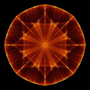
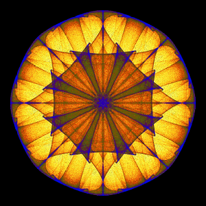
There are two basic ways to render a high-quality image. A high oversample level (16) and a low density (1-2) result in a finely-detailed, semi-transparent, three-dimensional “spun glass” appearance that often suggests motion; these images look best with simple color palettes. A moderate oversample level (4) and a high density (16+) result in a mostly solid image that tends to require a complex palette, which gives it a “stained glass” look. For a lower-resolution preview of either of the above, reduce the oversample level.
|
|
If the script is taking too long and you change your mind, click abort.
The information field displays the progress of the script. The final result consists of the number of generated points, the maximum number of hits that any subpixel received, the elapsed time, and histogram data showing how many subpixels got how many hits. The position of each histogram entry in the series is also given as a percentile of the total number of hits; the color palette is based on this number.
Last: apply a color palette. Several sample palettes are provided. Make your own by entering hex color and percentile pairs, one per line; then press redraw palette. A color picker is provided to find hex color values. Roll the mouse over the image and the percentile of the indicated point is displayed below; this can help to position colors in the palette. To apply the palette, press recolor the image; recoloring only takes a small fraction of the time that it took to render the image.
(The position numbers do not have to be percentiles; use any numbers and they will be normalized to 0-100. Omit the number and the color will be skipped. The entries do not have to be in order; you can reverse the numbers to reverse colors.)
Images differ in their pixel distributions; a given palette may need to be stretched in either direction for the best results.
When you are happy with the image, right-click the canvas to save it. Click save beside the parameter field to write the parameter set to the parameter field; replace “name” with a name, then copy and save it to a text file. Paste a saved parameter set into the field and click load to load it.